## Warning: package 'deSolve' was built under R version 4.3.1Migrate deSolve code to denim
Original code in deSolve
The model used for demonstrating the process of migrating code from
deSolve to denim is as followed
# --- Model definition in deSolve
transition_func <- function(t, state, param){
  with(as.list( c(state, param) ), {
      dS = -beta*S*I/N
      dI1 = beta*S*I/N - rate*I1
      dI2 = rate*I1 - rate*I2
      dI =  dI1 + dI2
      dR = rate*I2
      list(c(dS, dI, dI1, dI2, dR))
  })
}

# ---- Model configuration
parameters <- c(beta = 0.3, rate = 1/3, N = 1000)
initialValues <- c(S = 999, I = 1, I1 = 1, I2=0, R=0)

# ---- Run simulation
times <- seq(0, 100) # simulation duration
ode_mod <- ode(y = initialValues, times = times, parms = parameters, func = transition_func)

# --- show output
ode_mod <- as.data.frame(ode_mod)
head(ode_mod[-1, c("time", "S", "I", "R")])
## time S I R
## 2 1 998.6561 1.294182 0.04969647
## 3 2 998.2239 1.594547 0.18152864
## 4 3 997.6985 1.921416 0.38010527
## 5 4 997.0695 2.290735 0.63971843
## 6 5 996.3225 2.716551 0.96093694
## 7 6 995.4387 3.212577 1.34869352Model definition
Similar to deSolve, transitions between compartments in
denim can be defined using ordinary differential equations
(ODEs). However, denim extends it by providing the option
to directly express the dwell time distribution.
To utilize this option from denim, the user must first
identify which transitions can best describe the ones in their
deSolve model.
Identify distribution
# --- Model definition in deSolve
transition_func <- function(t, state, param){
  with(as.list( c(state, param) ), {

      # For S -> I transition, since it involves parameters (beta, N),
      # the best transition to describe this is using a mathematical formula
      dS = -beta*S*I/N

      # For I -> R transition, linear chain trick is applied --> implies Erlang distributed dwell time
      # Hence, we can use d_gamma from denim
      dI1 = beta*S*I/N - rate*I1
      dI2 = rate*I1 - rate*I2
      dI =  dI1 + dI2
      dR = rate*I2
      list(c(dS, dI, dI1, dI2, dR))
  })
}
With the transitions identified, the user can then define the model
in denim.
When using denim DSL, the model structure is given as a
set of key-value pairs where
key shows the transition direction between compartments in the format of
compartment -> out_compartment.value is either a built-in distribution function that describe the transition or a mathematical expression.
Model configurations
Similar to deSolve, denim also ask the
users to provide the initial values and any additional
parameters in the form of named vectors or named list.
For the example deSolve code, while the users can use
the initalValues from the deSolve code as is
(denim will ignore unused I1, I2
compartments as these sub-compartments will be automatically computed
internally), it is recommended to remove redundant compartments (in this
example, I1 and I2).
For parameters, since rate is already defined in the
distribution functions, the users only need to keep beta
and N from the initial parameters vector. We do not need to
specify the value for timeStep variable as this is a
special variable in denim and will be defined later on.
# remove I1, I2 compartments
denim_initialValues <- c(S = 999, I = 1, R=0)
denim_parameters <- c(beta = 0.3, N = 1000)
Initialization of sub-compartments: when
there are multiple sub-compartments (e.g., compartment I
consist of I1 and I2 sub-compartments), the
initial population is always assigned to the first sub-compartment. In
our example, since I = 1, denim will assign
I1 = 1 and I2 = 0.
There is also an option to distribute initial value across
sub-compartments based on the specified distribution. To do this, simply
set dist_init parameter of distribution function to
TRUE.
transitions <- denim_dsl({
S -> I = beta * S * I/N
I -> R = d_gamma(rate = 1/3, shape = 2, dist_init = TRUE)
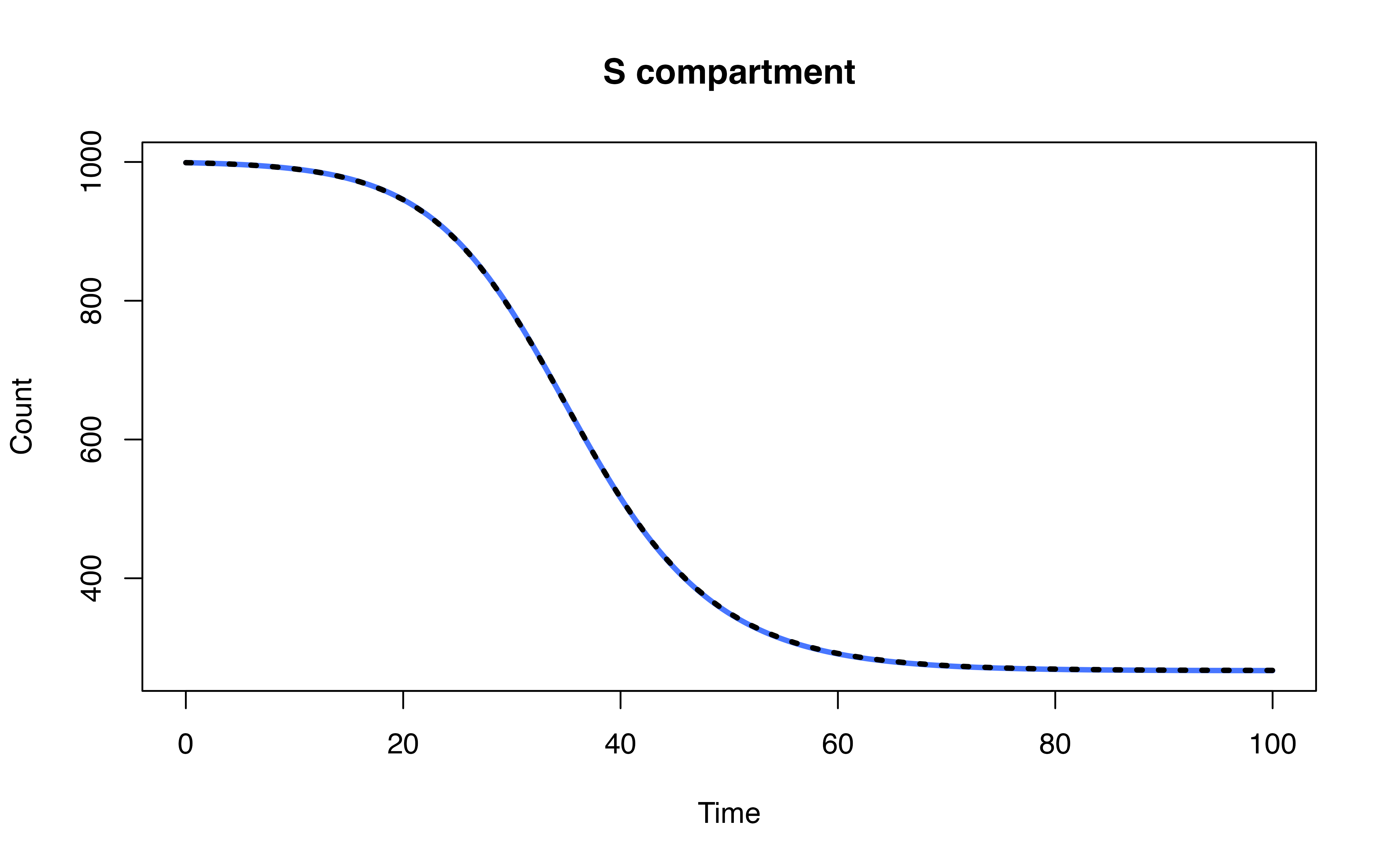
})However, for comparison purposes, we will keep this option
FALSE for the remaining of this demonstration.
Simulation
Lastly, the users need to define the simulation duration and time
step for denim to run. Unlike deSolve which
takes a time sequence, denim only require the simulation
duration and time step.
Since denim uses a discrete time approach, time step
must be set to a small value for the result to closely follow that of
deSolve (in this example, 0.01).
mod <- sim(transitions = transitions,
             initialValues = denim_initialValues,
             parameters = denim_parameters,
             simulationDuration = 100,
             timeStep = 0.01)

head(mod[mod$Time %% 1 == 0, ])
## Time S I R
## 1 0 999.0000 1.000000 0.00000000
## 101 1 998.6566 1.293759 0.04961535
## 201 2 998.2251 1.593725 0.18121212
## 301 3 997.7004 1.920189 0.37940195
## 401 4 997.0725 2.289061 0.63848007
## 501 5 996.3266 2.714365 0.95900520