transition to multiple states • denim

library(deSolve)

## Warning: package 'deSolve' was built under R version 4.3.1

library(denim)

1. Transition to multiple states in denim

Modelers may encounter many situations where individuals can transition from one compartment to multiple others, such as the SIRD model. There are 2 main approaches to handle this:

Model transitions as competing risks
Model as multinomial transition (outgoing population is split by a fixed proportion to transition to new compartments).

denim allows users to model both situations, while requiring minimal change to the code base to switch between 2 methods of modeling.

2. Multinomial in denim

2.1. Model definition

To specify the proportion that goes to each outgoing compartment, define the transition using the following syntax in model definition:

proportion * compartment -> out_compartment = [transition]

Note that the proportion here is the proportion of compartment that will end up in out_compartment at equilibrium.

Example: An SIRD model where 90% of infected can recover while the remaining 10% will die.

transitions <- denim_dsl({
  S -> I = beta * S * (I / N) * timeStep
  0.9 * I -> R = d_gamma(1/3, 2)
  0.1 * I -> D = d_exponential(0.1)
})

Mathematical formulation for the model

\[ \begin{cases} dS = -\beta S \frac{I}{N} \\ dIR_1 = 0.9 *\beta S \frac{I}{N} -\frac{1}{3}IR_1 \\ dIR_2 = \frac{1}{3}IR_1 - \frac{1}{3}IR_2 \\ dID = 0.1*\beta S \frac{I}{N} - 0.1*ID \\ dR = \frac{1}{3}IR_2 \\ dD = 0.1*ID \end{cases} \]

Proportion normalization

denim will automatically normalize the proportions if they don’t sum up to 1.

Example 2: The following model definition is equivalent to the one in Example 1

transitions <- denim_dsl({
  S -> I = beta * S * (I / N) * timeStep
  36 * I -> R = d_gamma(1/3, 2)
  4 * I -> D = d_exponential(0.1)
})

2.2. Example model

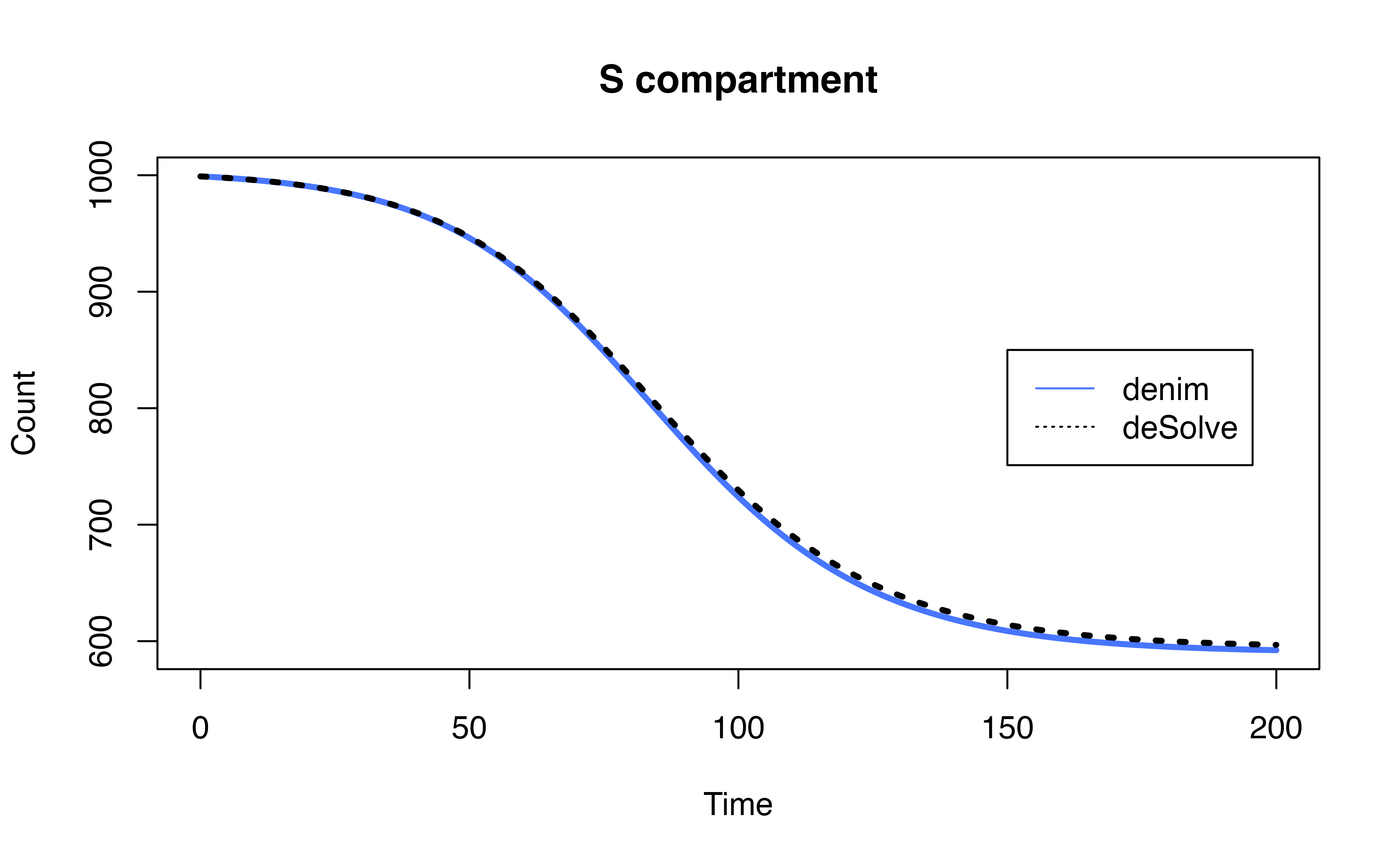
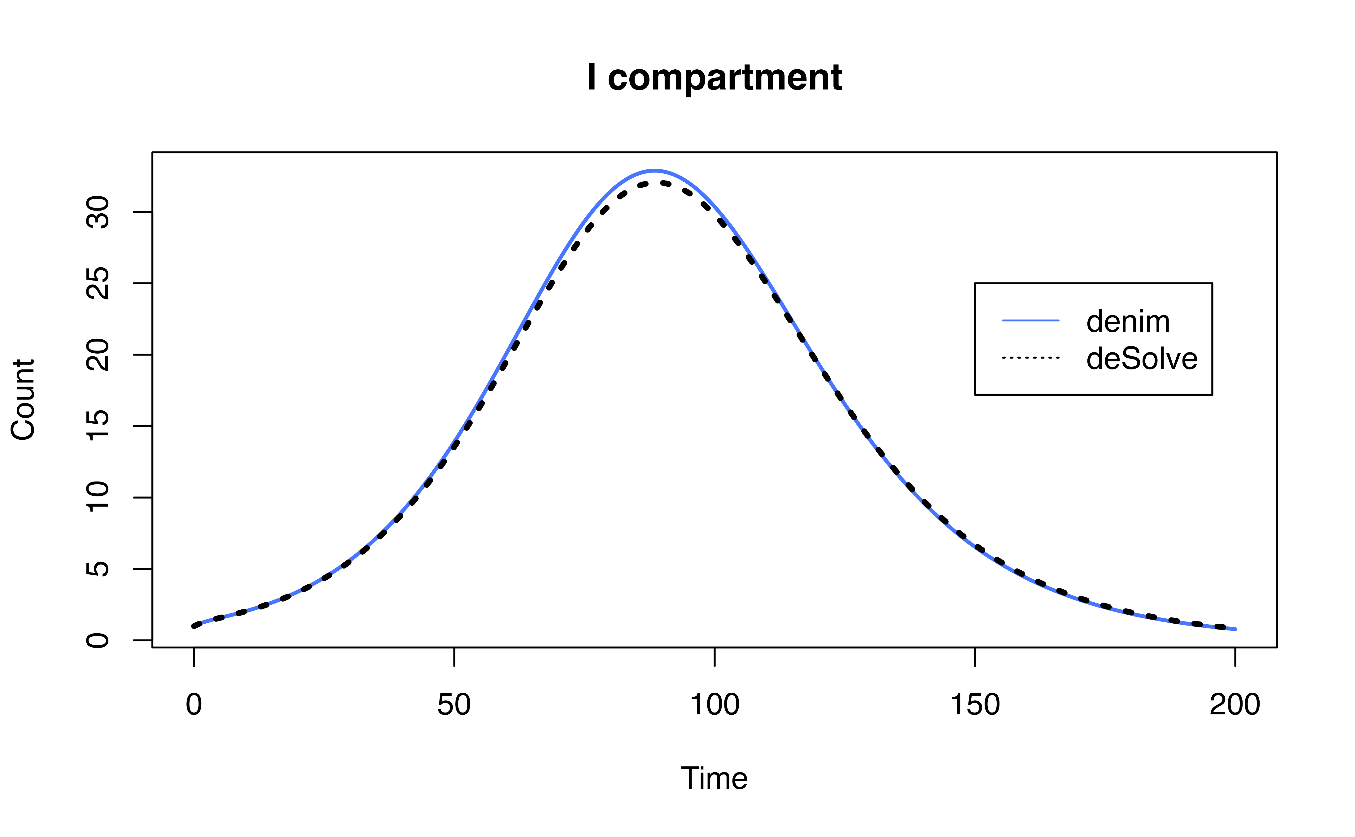
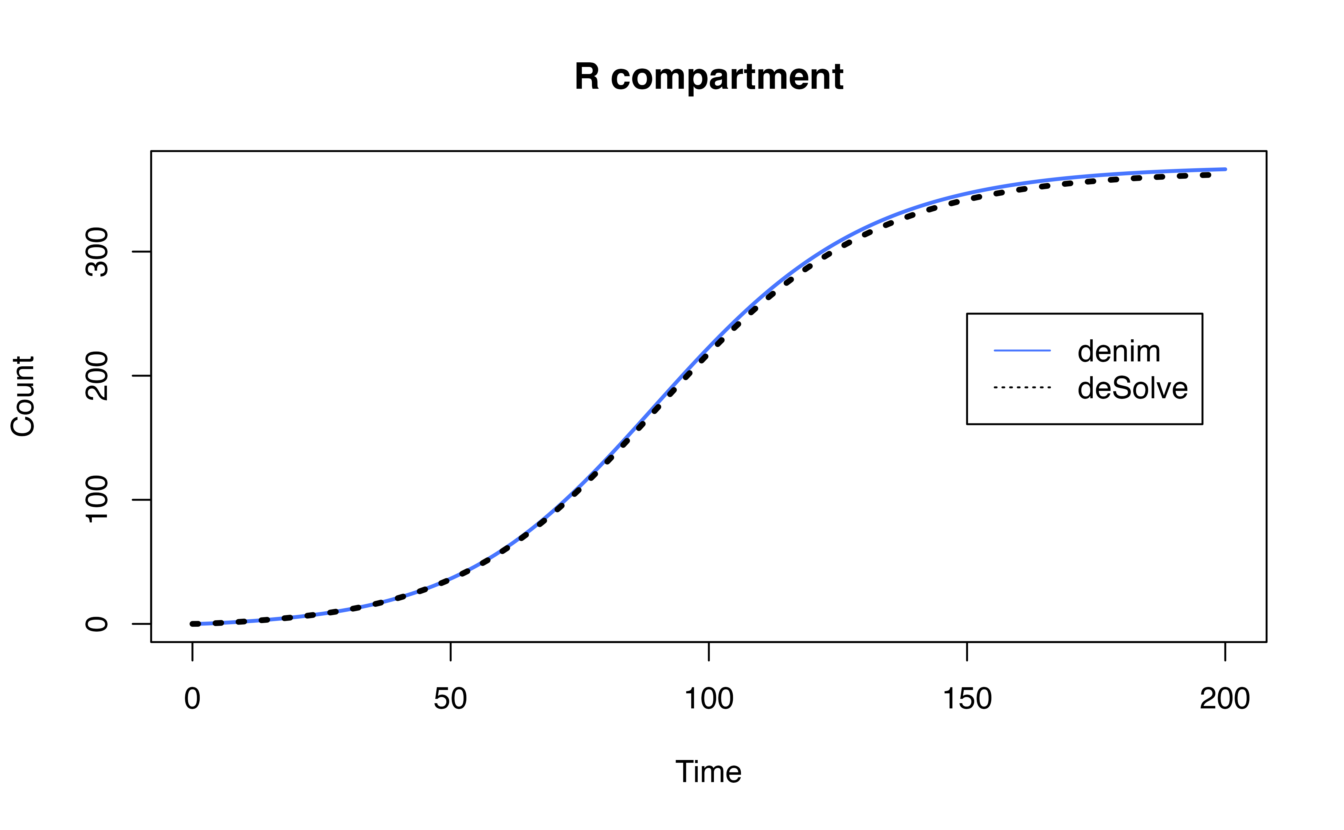
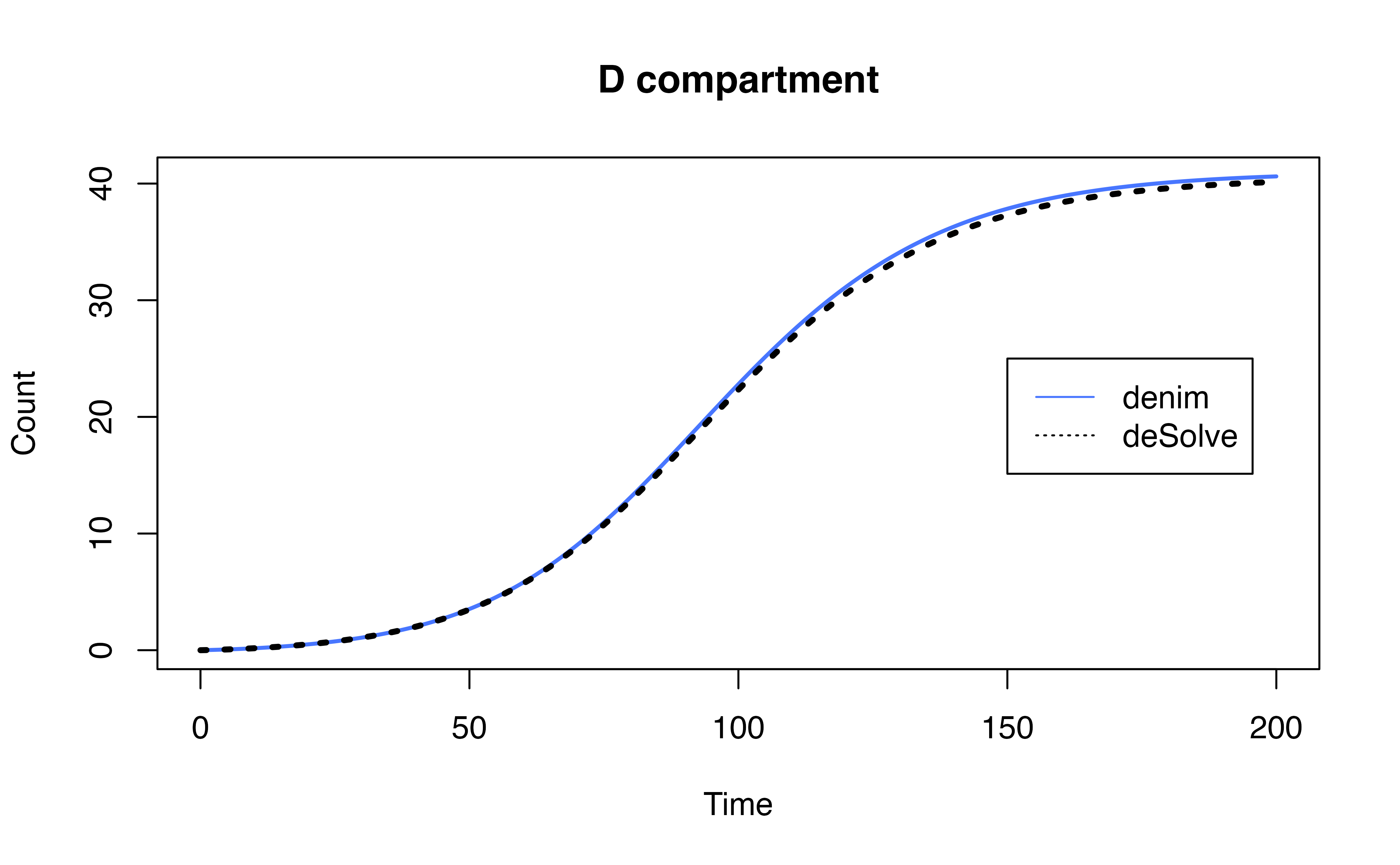
To further demonstrate the implementation of multinomial in denim, we provide the equivalent model implemented in deSolve and compare the output of 2 implementations.

Model definition in denim

# model in denim
transitions <- denim_dsl({
  S -> I = beta * S * (I / N) * timeStep
  0.9 * I -> R = d_gamma(1/3, 2)
  0.1 * I -> D = d_exponential(0.1)
})

denimInitialValues <- c(
  S = 999, 
  I = 1, 
  R = 0,
  D = 0
)

Equivalent model definition in deSolve

# model in deSolve
transition_func <- function(t, state, param){
  with(as.list( c(state, param) ), {

      dS = - beta * S * (IR1 + IR2 + ID)/N
      # apply linear chain trick for I -> R transition
      # 0.9 * to specify prop of I that goes to I->R transition
      dIR1 = 0.9 * beta * S * (IR1 + IR2 + ID)/N - rate*IR1
      dIR2 = rate*IR1 - rate*IR2
      dR = rate*IR2 
      
      # handle I -> D transition
      # 0.1 * to specify prop of I that goes to I->D transition
      dID = 0.1 * beta * S * (IR1 + IR2 + ID)/N - exp_rate*ID
      dD = exp_rate*ID
      list(c(dS, dIR1, dIR2, dID, dR, dD))
  })
}

desolveInitialValues <- c(
  S = 999, 
  # note that internally, denim also allocate initial value based on specified proportion
  IR1 = 0.9,
  IR2 = 0,
  ID = 0.1, 
  R = 0,
  D = 0
)

Run simulation and compare

Model settings

parameters <- c(
  beta = 0.2,
  N = 1000,
  rate = 1/3,
  exp_rate = 0.1
)

simulationDuration <- 200
timeStep <- 0.05

Run model

# --- run denim model ---- 
mod <- sim(transitions = transitions, 
           initialValues = denimInitialValues, 
           parameters = parameters, 
           simulationDuration = simulationDuration, 
           timeStep = timeStep)

# run deSolve model
times <- seq(0, simulationDuration)
ode_mod <- ode(y = desolveInitialValues, times = times, parms = parameters, func = transition_func) 
ode_mod <- as.data.frame(ode_mod)
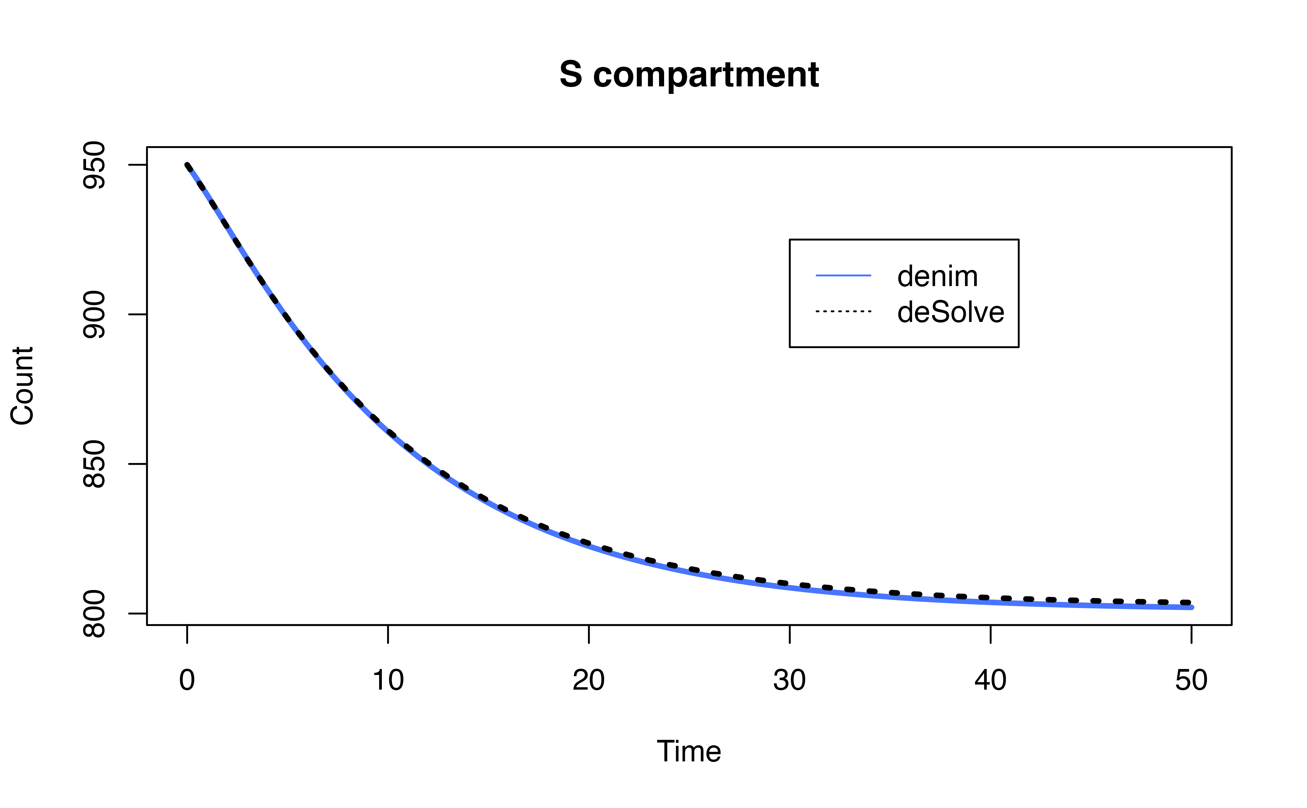
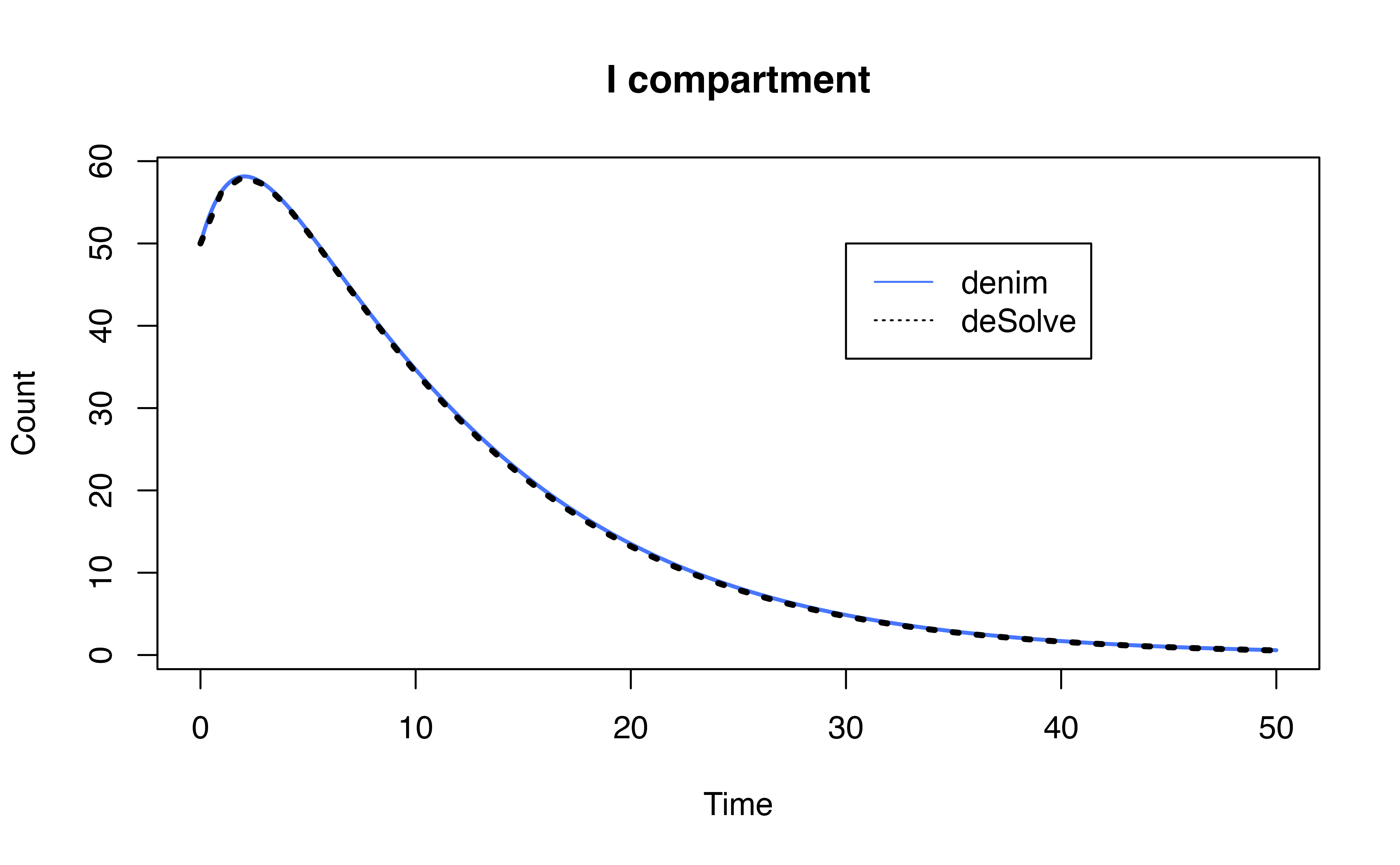
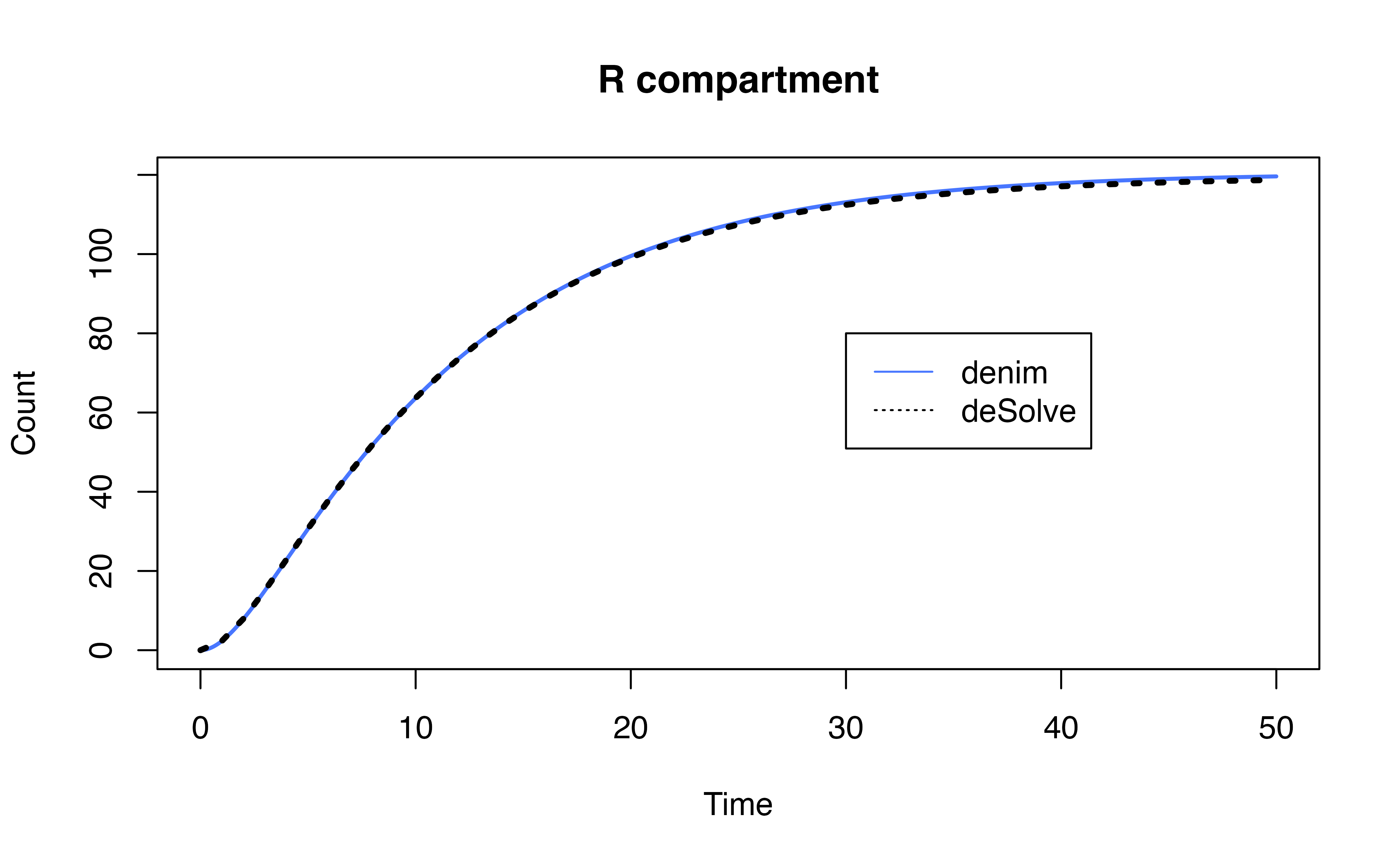
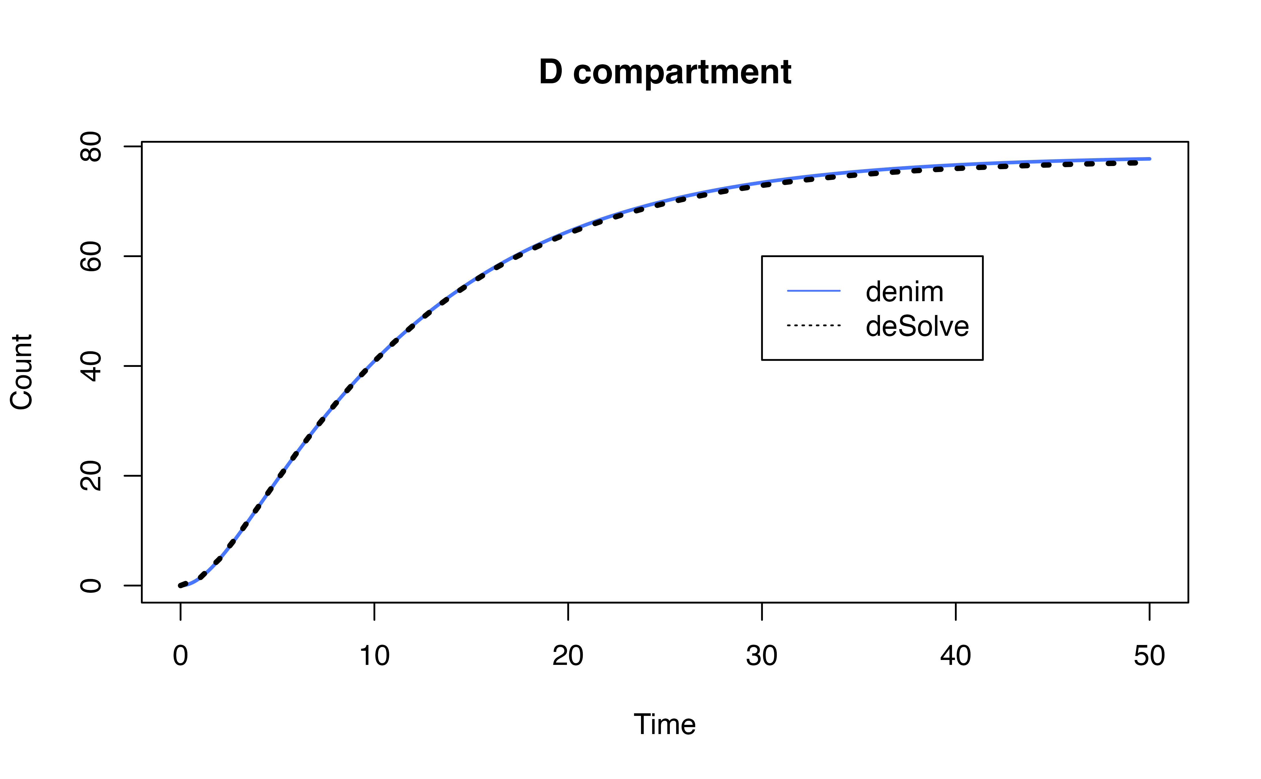
ode_mod$I<- rowSums(ode_mod[, c("IR1", "IR2", "ID")])

Output Comparison

3. Competing risks in denim

3.1. Model definition

When there are multiple transitions from one compartment and no proportions are specified, denim will automatically treat these transitions as competing risks.

Example: the following model definition will treat I->R and I->D as competing risks.

transitions <- denim_dsl({
  S -> I = beta * S * (I / N) * timeStep
  I -> R = d_gamma(rate = 1/3, shape = 2)
  I -> D = d_gamma(rate = 1/4, shape = 2)
})

3.2. Example model

To further demonstrate the implementation of competing risks in denim, we provide the equivalent model implemented in deSolve and compare the output of 2 implementations.

Model definition in denim

transitions <- denim_dsl({
  S -> I = beta * S * (I / N) * timeStep
  I -> R = d_gamma(rate = 1/3, shape = 2)
  I -> D = d_gamma(rate = 1/4, shape = 2)
})

denimInitialValues <- c(
  S = 950, 
  I = 50, 
  R = 0, 
  D = 0
)

Equivalent model definition in deSolve

transition_func <- function(t, state, param){
  with(as.list( c(state, param) ), {
    dS = - beta * S * (I1 + I2 + IR + ID)/N

    dI1 = beta * S * (I1 + I2 + IR + ID)/N - (rate+d_rate)*I1

    dIR = rate*I1 - (d_rate + rate)*IR
    dID = d_rate*I1 - (d_rate + rate)*ID

    dI2 = d_rate*IR + rate*ID - (d_rate + rate)*I2

    dR = rate*IR + rate*I2
    dD = d_rate*ID + d_rate*I2

    list(c(dS, dI1, dIR, dID, dI2, dR, dD))
  })
}

desolveInitialValues <- c(
  S = 950, 
  I1 = 50,
  IR = 0,
  ID = 0,
  I2 = 0,
  R = 0,
  D = 0
)

Run simulation and compare

Model settings

parameters <- c(
  beta = 0.2,
  N = 1000,
  rate = 1/3,
  d_rate = 1/4
)

simulationDuration <- 50
timeStep <- 0.05

Run model

# run denim model
mod <- sim(transitions = transitions, 
           initialValues = denimInitialValues, 
           parameters = parameters, 
           simulationDuration = simulationDuration, 
           timeStep = timeStep)

# run deSolve model
times <- seq(0, simulationDuration)
ode_mod <- ode(y = desolveInitialValues, times = times, parms = parameters, func = transition_func) 
ode_mod <- as.data.frame(ode_mod)
ode_mod$I <- rowSums(ode_mod[,c("I1", "ID", "IR", "I2")])