Model definition in denim
In denim, model is defined by a set of transitions between compartments. Each transition is provided in the form of a key-value pair, where:
key show the transition direction between 2 compartments.
value is an expression that describe the transition, either as a rate given by a math expression or as a distribution of dwell-time in the origin compartment. This distribution can be specified parametrically using the built-in distribution function or through providing of histogram numeric values.
These key-value pairs can be provided in 2 ways
Using denim domain-specific language (DSL).
Define as a
listin R.
Denim DSL
In denim, each line of code must be a transition. The syntax for defining a transition in denim DSL is as followed:
from -> to = [transition]
Model definition written in denim DSL must be parsed by the function
denim_dsl()
Math expression
For math expression, some basic supported operators include:
+ for addition, - for minus, *
for multiplication, / for division, ^ for
power. The users can also define additional model parameters in the math
expression.
Math expressions in denim are parsed using muparser. For a full list of operators, visit the muparser website at https://beltoforion.de/en/muparser/features.php.
Distribution functions
Several built-in functions are provided to describe transitions based on the distribution of dwell time:
For parametric distributions:
d_lognormal(),d_gamma(),d_weibull(),d_exponential()For non-parametric distributions:
nonparametric()
Each of these functions accepts either fixed numerical values or model parameters as inputs for their distributional parameters.
Define a classic SIR model
A classic SIR model can be defined in denim as followed
sir_model <- denim_dsl({
  S -> I = beta * (I/N) * S
  I -> R = d_exponential(rate = gamma)
})
denim_dsl() parses the given expression and return an R
list as followed.
sir_model
#> $`S -> I`
#> [1] "beta * (I/N) * S"
#>
#> $`I -> R`
#> Discretized exponential distribution
#> Rate = gamma
#>
#> attr(,"class")
#> [1] "denim_transition"
In this example, model parameters are: N,
beta, gamma.
Users can also choose to provide fixed values as the distributional parameter as followed.
sir_model <- denim_dsl({
  S -> I = beta*(I/N)*S
  I -> R = d_exponential(rate = 1/4)
})
Similar to R, the users can also add comments in denim DSL by
starting the comment with # sign.
sir_model <- denim_dsl({
  # this is a comment
  S -> I = beta*(I/N)*S
  I -> R = d_exponential(rate = 1/4) # this is another comment
})
Run model
To run the model, the users must provide:
Values for model parameters (in this example,
N,beta, andgamma).Initial population for the compartments.
Simulation configurations.
Parameters and initial values can be defined as named vectors or named lists in R.
# parameters for the model
parameters <- c(
  beta = 0.4,
  N = 1000,
  gamma = 1/7
)
# initial population for each compartment
initValues <- c(
  S = 999,
  I = 50,
  R = 0
)
Simulation configurations are provided as parameters for
sim() function which runs the model, where:
timeStepis the duration of each time step in the model.simulationDurationis the duration to run the simulation.
mod <- sim(sir_model,
    parameters = parameters,
    initialValues = initValues,
    timeStep = 0.01,
    simulationDuration = 40)
Time varying transition
variable time is a special variable in denim for time
varying transition (e.g. for modeling seasonality). Note that this
variable can ONLY be used within math expression.
Example: time varying transition
time_varying_mod <- denim_dsl({
  A -> B = 20 * (1+cos(omega * time))
})

# parameters for the model
parameters <- c(
  omega = 2*pi/10
)
# initial population for each compartment
initValues <- c(A = 1000, B = 0)

mod <- sim(time_varying_mod,
    parameters = parameters,
    initialValues = initValues,
    timeStep = 0.01,
    simulationDuration = 40)

plot(mod, ylim = c(0, 1000))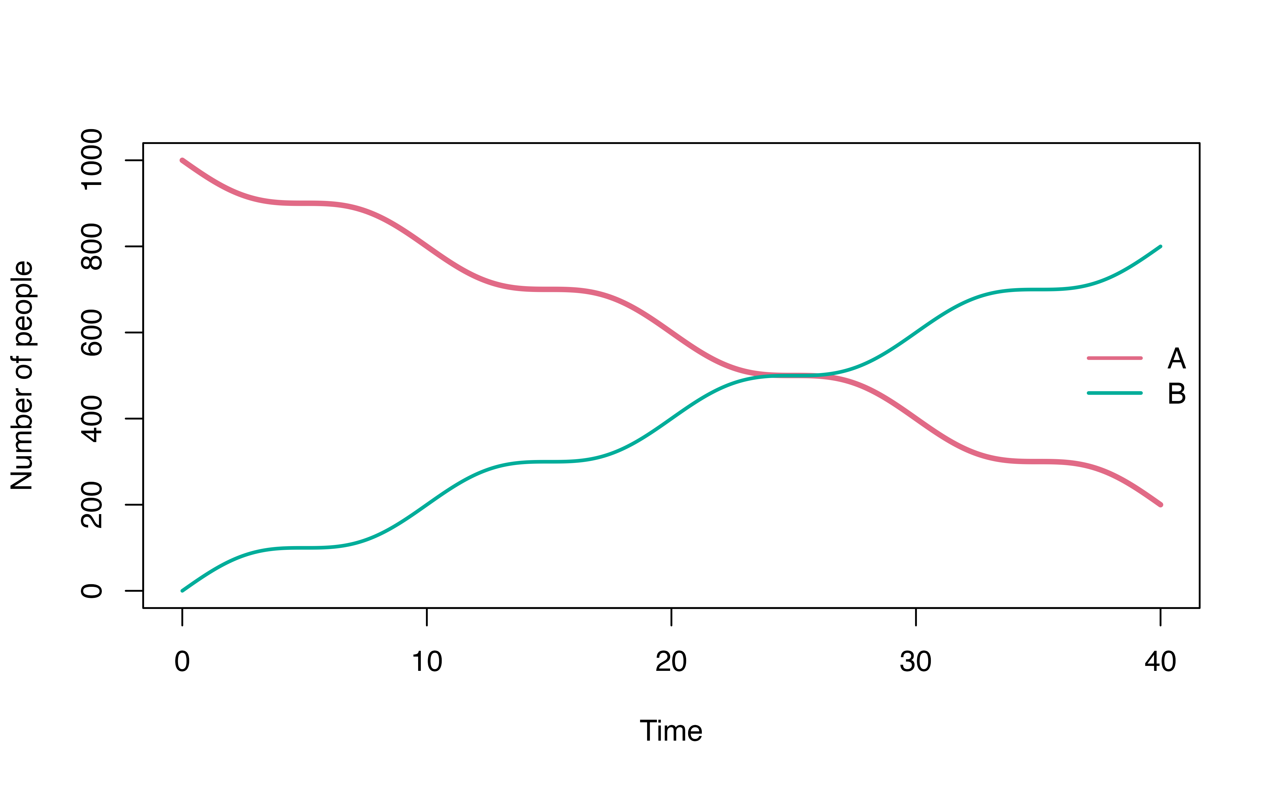
R list
Users can define the model structure directly as a list in R. For example, the SIR model from previous example can be represented as followed.
sir_model_list <- list(
  "S -> I" = "beta * (I/N) * S",
  "I -> R" = d_exponential(rate = "gamma")
)

sir_model_list
#> $`S -> I`
#> [1] "beta * (I/N) * S"
#>
#> $`I -> R`
#> Discretized exponential distribution
#> Rate = gamma
Note that the transitions (S -> I,
I -> R), mathematical expression
(beta * (I/N) * S), and the model parameter
(gamma) must now be provided as strings.
We can then run the model in the same manner as previously demonstrated.
# parameters for the model
parameters <- c(
  beta = 0.4,
  N = 1000,
  gamma = 1/7
)
# initial population for each compartment
initValues <- c(
  S = 999,
  I = 50,
  R = 0
)
# run the simulation
mod <- sim(sir_model_list,
    parameters = parameters,
    initialValues = initValues,
    timeStep = 0.01,
    simulationDuration = 40)
# plot output
plot(mod, ylim = c(1, 1000))
When should I define model as a list in R?
While denim DSL offers cleaner and more readable syntax to define model structure, using R list may be more familiar to R users and better suited for integration to a more R-centric workflow.
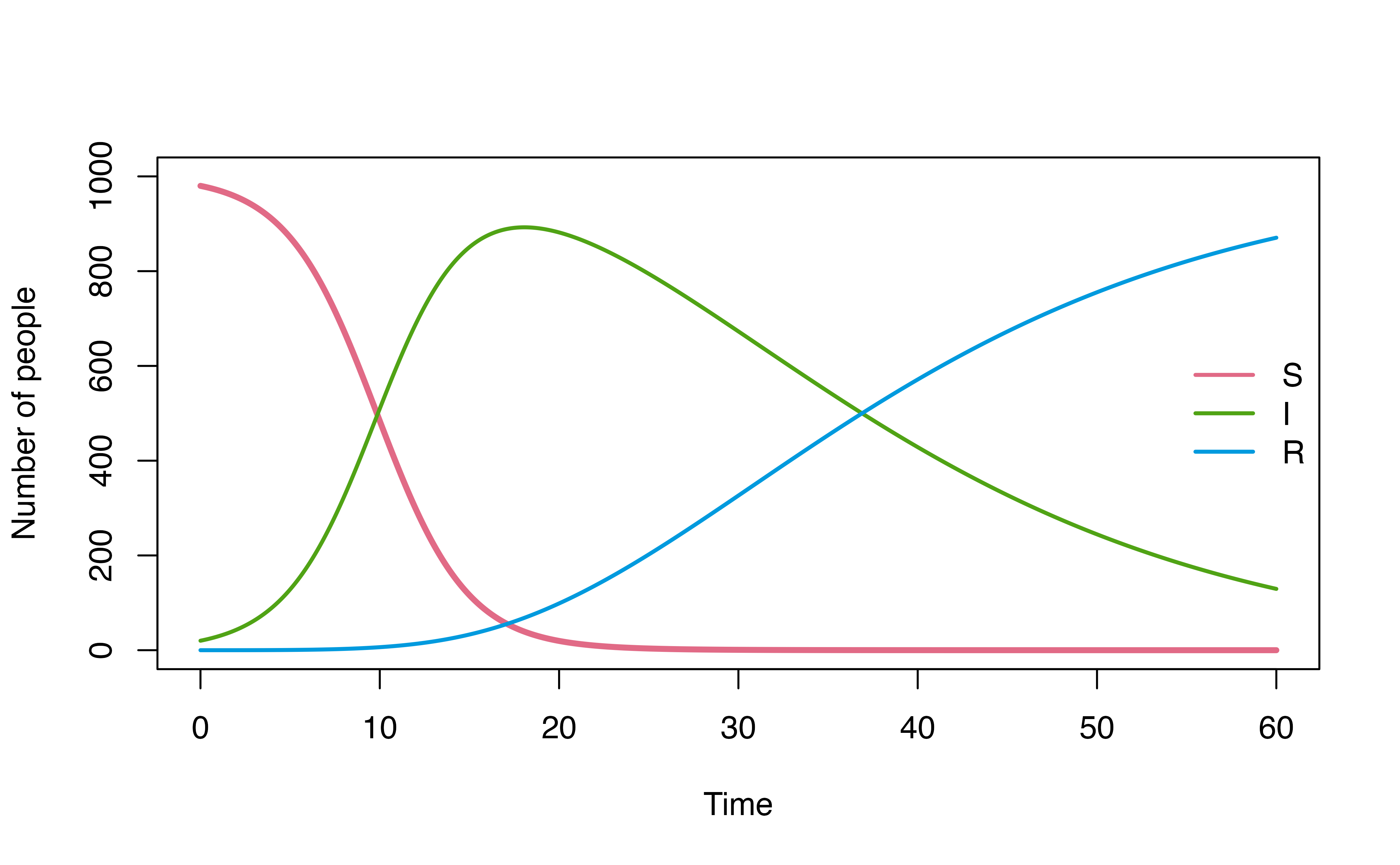
For example, consider a use case below, where we explore how model
dynamics change under three different I -> R dwell time
distributions (d_gamma, d_weibull,
d_lognormal) using map2.
library(tidyverse)
# configurations for 3 different I->R transitions
model_config <- tibble(
  IR_dists = c(d_gamma, d_weibull, d_lognormal),
  IR_pars = list(c(rate = 0.1, shape = 3), c(scale = 5, shape = 0.3), c(mu = 0.3, sigma = 2))
)

walk2(
  model_config$IR_dists, model_config$IR_pars, \(dist, par){
    transitions <- list(
      "S -> I" = "beta * S * (I / N)",
      # This is not applicable when using denim_dsl()
      "I -> R" = do.call(dist, as.list(par))
    )

    # model settings
    denimInitialValues <- c(S = 980, I = 20, R = 0)
    parameters <- c(
      beta = 0.4,
      N = 1000
    )

    # compare output
    mod <- sim(transitions = transitions,
               initialValues = denimInitialValues,
               parameters = parameters,
               simulationDuration = 60,
               timeStep = 0.05)

    plot(mod, ylim = c(0,1000))
})