Reproduction number

Figure from Corona confusion: What do all the numbers mean?, by Deutsche Welle.
The reproduction number, \(R\), is the average number of secondary cases of disease caused by a single infected individual over his or her infectious period (Cori et al., 2013).
Basic reproduction number \(R_0\)
Definition 1 \(R_0\) (pronounced /R naught/) is the average number of individuals infected by each infectious individual in a fully susceptible population (Vegvari et al., 2022). In short, \(R_0\) is the \(R\) in a fully susceptible population, the maximum \(R\) in a population.
The basic reproduction number is sometimes called the basic reproductive number or basic reproductive ratio (Driessche, 2017).
Estimations of the R0 value are often calculated as a function of 3 primary parameters (Chitnis, 2017; Jones, 2007):
\[R_0 = \begin{pmatrix} \text{Number of} \\ \text{contacts} \\ \text{per unit time} \end{pmatrix} \times \begin{pmatrix} \text{Probability of} \\ \text{transmission} \\ \text{per contact} \end{pmatrix} \times \begin{pmatrix} \text{Duration} \\ \text{of} \\ \text{infectious} \end{pmatrix}\]
- For many vaccine-preventable diseases, \(R_0\) values were calculated long ago in history. For example, measles \(R_0\) values of 12-18 are based on data from 1912-1928 in the United States (\(R_0 = 12.5\)) and 1944-1979 in England and Wales (\(R_0 = 13.7-18.0\)). For pertussis, the original data sources are 1908-1917 in the United States (\(R_0 = 12.2\)) and 1944-1979 in England and Wales (\(R_0 = 14.3-17.1\)). Human contact patterns in the past are extremely unlikely to match present day epidemiological realities. However, historical \(R_0\) values are so frequently cited that new \(R_0\) values using modern data might be dismissed if they fall outside the old range. Public health decisions should be made using up-to-date \(R_0\) values (Delamater et al., 2019).
- \(R_0\) is not a biological constant for a pathogen, and \(R_0\) cannot be modified through vaccination campaigns (Delamater et al., 2019). In fact, more than 20 different \(R_0\) values (range 5.4-18) were reported for measles in a variety of study areas and periods, and a review in 2017 identified feasible measles \(R_0\) values of 3.7-203.3 (Delamater et al., 2019).
- \(R_0\) estimates in the early phase may not be representative for the population if the group of initial transmitters is atypical (Vegvari et al., 2022) (e.g. monkeypox).
- \(R_0\) may be incorrectly estimated if asymptomatic individuals are not counted or recognised, and their epidemiologically relevant behaviour differs from that of symptomatic individuals (Vegvari et al., 2022).
Effective reproduction number \(R_e\)
Definition 2 \(R_e\) is the average number of secondary cases generated by each infectious individual throughout their infectious period in a population that may be partially immune (Wallinga & Lipsitch, 2006).
Let \(s\) be the proportion of the population that is susceptible.
\[R_e = s \times R_0\]
Effective reproduction number at time \(t\) \(R_t\)
Definition 3 \(R_e(t)\) (Knight & Mishra, 2020) or \(R_t\) is the average number of secondary cases generated by one infected person at time \(t\) during the outbreak, where some individuals may no longer be susceptible (Gostic et al., 2020).
A public health control strategy will end an outbreak if it can keep \(R_t\) below 1. The level of immunity at which \(R_t = 1\) is the herd immunity threshold (Vegvari et al., 2022).
At the beginning of an outbreak, we can estimate \(R_0\) when the whole population is fully susceptible. As the outbreak progresses, the number of susceptible individuals decreases, leading to a decline in \(R_0\). This adjusted value is referred to as \(R_t\) (if we want to measure at each time \(t\)). At the peak of the epidemic curve, \(R_t = 1\). After this peak, \(R_t\) continues to decrease, resulting in a decline in the number of new cases and the epidemic curve going down.
\(R_t\) can be defined in 2 ways:
- Instantaneous reproduction number (\(R_t^i\)): the average number of individuals someone infected at time \(t\) would infect if conditions remained unchanged (Green et al., 2022).
- Case reproduction number (\(R_t^c\)): the average number of people an individual infected at time t actually infects, which will depend on changes in policy or behavior over the period of that cohort’s infection, and can only be estimated in retrospect (Green et al., 2022).
Instantaneous reproduction number \(R_t^i\)

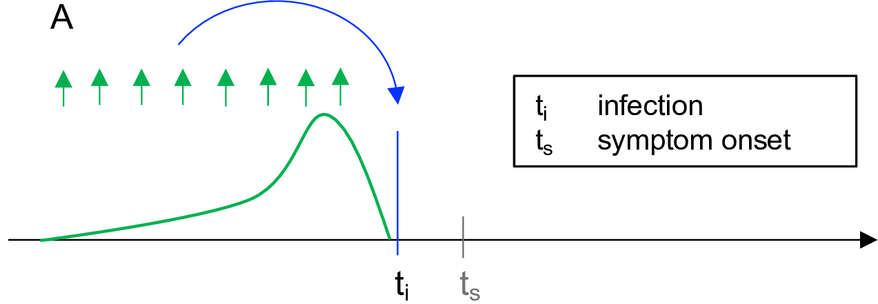
Figure illustrates the Cori method (Gostic et al., 2020).
Measures transmission at a specific point in time (Gostic et al., 2020). The instantaneous reproduction number quantifies the number of new infections at a single point in time \(t_i\) (blue arrow), using the number of infections in the previous generation (green arrows) and their current infectiousness (green curve) (Gostic et al., 2020). The analyses can be done near real-time.
Methods to estimate instantaneous reproduction number includes Cori and colleagues (Cori et al., 2013) (the best for near real-time estimation (Gostic et al., 2020)), and Bettencourt and Ribeiro (Bettencourt & Ribeiro, 2008) (use with caution because they implicitly assume the generation interval follows an exponential distribution, as in SIR model, which does not include alatent period).
Case reproduction number \(R_t^c\)

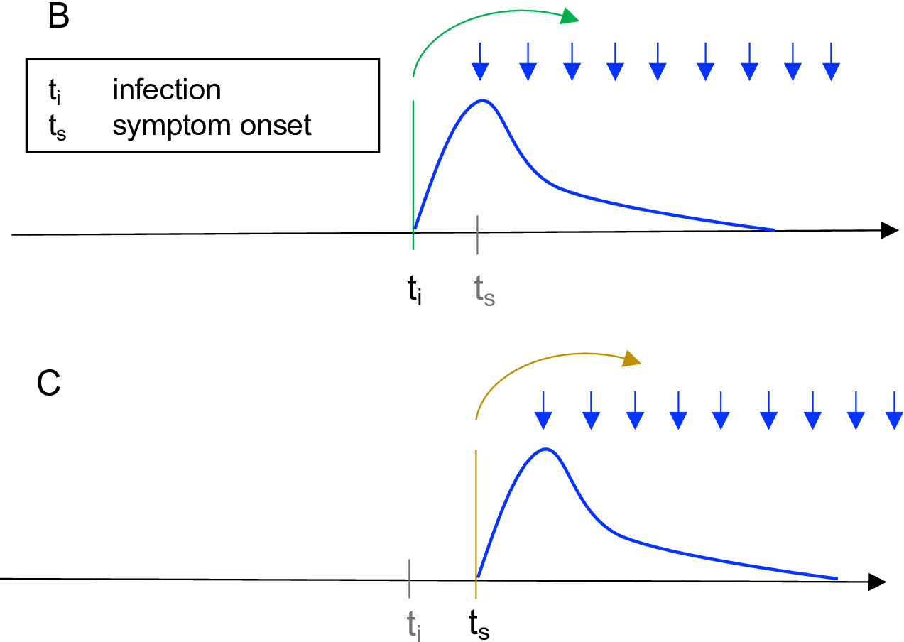
Figure illustrates the Wallinga and Teunis method (Gostic et al., 2020).
Measures transmission by a specific cohort of individuals (Gostic et al., 2020). A cohort is a group of individuals with the same date of infection or the same date of symptom onset. The case reproduction number is the average number of new infections that an individual who becomes infected on day \(t_i\) (green arrows in B) or symptomatic on day \(t_s\) (yellow arrows in C) will eventually go on to cause (blue downward arrows in B and C). It is a more natural choice for analyses that consider heterogeneity among individuals (Gostic et al., 2020).
Methods to estimate instantaneous reproduction number includes Wallinga and Teunis method (Wallinga & Teunis, 2004).
Growth rate \(r\) and basic reproduction number \(R_0\)
In the initial phase of an epidemic where the population is completely susceptible, incidence increase exponentially.
The exponential growth rate \(r\) is defined as the per capita change in number of new cases per unit of time (Wallinga & Lipsitch, 2006). Let \(C_0\) be the incidence at time \(t = 0\). For continuous time \(t\), the incidence at time \(t\) is given by:
\[C_t = C_0 e^{rt}\]
Let \(M\) is the money you have at time \(t = 0\), \(r\) is the annual interest rate. The money you have after each year would be:
\[\begin{align} M_1 & = M_0 + r M_0 = M_0 (1 + r) \\ M_2 & = M_1 + r M_1 = M_1 (1 + r) \\ & = M_0 (1 + r)(1 + r) = M_0 (1 + r)^2 \\ M_3 & = M_2 + r M_2 = M_2 (1 + r) \\ & = M_0 (1 + r)^2(1 + r) = M_0 (1 + r)^3 \\ & \cdots \\ M_t & = M_0 (1 + r)^t \end{align}\]
Now we imagined that, instead of paying interest once a year at a rate of \(r\), a bank might add interest twice a year at the rate \(\frac{r}{2}\), or three times a year at the rate \(\frac{r}{3}\). In general, we considered interest added \(n\) times a year at the rate of \(\frac{r}{n}\). In this case, each year your money is:
\[M_t = M_0 \left(1 + \frac{r}{n} \right)^{nt}\]
When \(n\) is very large and thus \(\frac{r}{n}\) is very small, we can prove that:
\[\lim_{n \to \infty} \left(1 + \frac{r}{n}\right)^{n} \approx e^r\]
Proof
\[L = \lim_{n \to \infty} \left(1 + \frac{r}{n}\right)^{n}\]
Take the natural logarithm:
\[\log L = \log \left[ \lim_{n \to \infty} \left(1 + \frac{r}{n}\right)^n \right]\]
Since the natural logarithm is a continuous function, we can bring the limit inside the logarithm.
\[\begin{align} \log L & = \lim_{n \to \infty} \log \left[ \left(1 + \frac{r}{n}\right)^n \right] \\ & = \lim_{n \to \infty} n \log \left(1 + \frac{r}{n} \right) \end{align}\]
For small values of \(x\), we can approximate \(\log(1 + x) \approx x - \frac{x^2}{2} + \frac{x^3}{3} - \cdots\). When \(x\) is very small, higher-order terms become negligible, so: \[\log \left(1 + \frac{r}{n}\right) \approx \frac{r}{n}\]
Substitute this approximation into \(L\):
\[\log L \approx \lim_{n \to \infty} n \left( \frac{r}{n} \right) = \lim_{n \to \infty} r = r\]
Therefore:
\[\begin{align} \log L & \approx r \\ \Leftrightarrow L & \approx e^r \\ \Leftrightarrow \lim_{n \to \infty} \left(1 + \frac{r}{n}\right)^{n} & \approx e^r \end{align}\]
Therefore:
\[M_t = M_0 \left(1 + \frac{r}{n} \right)^{nt} \approx M_0 e^{rt}\]
We start with \(C_0\) infected individuals, each infects \(R_0\) individuals after generation time \(T_g\). The number of infected individuals will be:
\[\begin{align} C_{T_g} & = C_0 R_0 \end{align} \tag{1}\]
We also proved that:
\[\begin{align} C_t & = C_0 e^{rt} \\ \Leftrightarrow C_{T_g} & = C_0 e^{rT_g} \end{align}\]
Substitute Equation 1, we have:
\[\begin{align} C_0 R_0 & = C_0 e^{rT_g} \\ \Leftrightarrow R_0 & = e^{rT_g} \end{align}\]
We can prove that:
\[R_0 = e^{rT_g} \approx 1 + rT_g\]
Expand \(e^x\) using the Taylor series:
\[e^x = 1 + x + \frac{x^2}{2!} + \frac{x^3}{3!} + \cdots\]
Substitute \(x\) with \(rT_g\) in the Taylor series expansion:
\[e^{rT_g} = 1 + rT_g + \frac{{rT_g}^2}{2!} + \frac{{rT_g}^3}{3!} + \cdots\]
For small values of \(rT_g\), \(\frac{{rT_g}^2}{2!}\), \(\frac{{rT_g}^3}{3!}\) become very small and can be neglected:
\[e^{rT_g} \approx 1 + rT_g\]